Balancing Frequencies and Pixels in Flow Matching
1LIX, École Polytechnique ·
2AMIAD ·
3LIGM, École des Ponts ·
4UC Berkeley
*Equal contribution †Equal supervision
TL;DR
Learn the frequencies first, then the pixels.
Natural images put most of their energy in low frequencies, so pixel-space losses spend most of their learning signal there and pick up textures and edges late. We propose the Focal Log-Frequency Loss (f-loss), which balances the training signal across the spectrum, and a schedule (fv-loss) that starts in frequency space and hands over to the standard pixel v-loss. It is a drop-in replacement for flow matching losses that speeds up convergence by up to 40% and requires no architectural change.
Guess the real image!
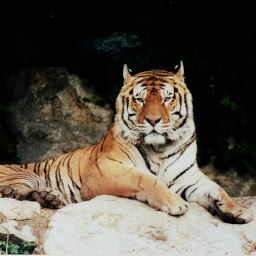
Two of these eight images are real ImageNet photos; the other six are generated by a pixel-space model trained with our fv-loss. Click the two you think are real.
1 · The problem
Pixel losses are spectrally biased
Natural images follow a \(1/f^2\) power spectrum: most of the signal energy lies in the low frequencies that describe global structure, while high frequencies carry sparse but structured details such as edges and textures. Flow matching with \(\boldsymbol{x}\)-prediction (as in JiT) trains with a pixel-space regression, the v-loss:
Every pixel error counts the same. By Parseval, this equals a squared error over Fourier coefficients, so the large low-frequency residuals dominate the optimization signal. Pick an image below to see how much each frequency octave contributes to the loss early in training, when the residual is roughly the image itself.
This bias shows in what a trained model generates. We compare the radially averaged power spectrum of images from a v-loss model with that of real ImageNet images. Low and mid frequencies are overestimated by about 20%, while high frequencies are underestimated, with a deficit that grows toward the Nyquist limit and reaches nearly −60%. The deficit is still there at the end of training.
Relative deviation of the generated power spectrum from real images throughout training (v-loss, JiT).
2 · Method
The Focal Log-Frequency Loss
We compute the residual in the Fourier domain, with \(e_{u,v} = |\mathcal{F}_\text{pred}(u,v) - \mathcal{F}_\text{target}(u,v)|\), and reweight it:
- Timestep weight: inherited unchanged from the v-loss, so the dynamics across timesteps stay the same.
- Adaptive focal weight: each per-frequency residual is normalized by the largest residual, under a stop-gradient. This avoids wide variations in magnitude between samples.
- Log compression: prevents any single frequency from monopolizing the loss. Like a continuous Laplacian pyramid, it gives every doubling of frequency equal weight.
Frequencies converge first, pixels catch up
The f-loss dominates early in training and converges significantly faster than the v-loss. However, the v-loss surpasses the f-loss later in training. The f-loss is insensitive to phase, which carries the exact spatial location of edges and textures, while the v-loss directly supervises pixel values and is better suited to locking sharp edges into exact pixel locations. Frequency supervision is the binding constraint early on, and pixel supervision becomes more effective as training progresses.
Guided FID during training, JiT-B/16 on ImageNet 256².
From frequencies to pixels: the fv-loss
We combine both objectives with a sigmoid schedule \(\lambda(s)\) that decays from 1 to 0 and is centered at the observed crossover point \(s^\star\):
Guided FID (JiT-B/16, ImageNet 256²)
Loss weights
3 · Watching models learn
Textures appear tens of thousands of steps earlier
Same class, same seed, same architecture; only the loss differs. Scrub through early training. The f-loss model renders the hay on the thatched roof and the knit of the mittens early, while the v-loss model first concentrates on sharp object boundaries.
4 · Results
Wall-clock speed-up
The f-loss computes a 2D FFT at every training step, which adds computational overhead. To check that this does not cancel the convergence speed-up, we measure the total wall-clock time for training JiT-B for 400k steps. Compared to the v-loss baseline (432.0 min), the f-loss adds +4% (453.1 min) and the fv-loss adds +14% (492.3 min), since it computes and backpropagates both losses at each step. At the 100-minute mark, the v-loss is temporarily ahead because the fv-loss has completed fewer steps (78k vs. 90k). The fv-loss overtakes it by the 200-minute mark, and from 300 minutes onward its convergence speed-up more than compensates for the added cost.
Guided FID vs. wall-clock training time, JiT-B/16. Labels give the training step reached at 400 minutes.
Convergence across model sizes
FID across training epochs for JiT-B/16, JiT-L/16 and JiT-XL/16, in both unguided and guided settings. The fv-loss outperforms the v-loss baseline across all model sizes from the earliest evaluations. The gap is largest in the early epochs and narrows as training progresses, consistent with our observation that frequency supervision is most valuable early in training.
JiT-B/16
JiT-L/16
JiT-XL/16
ImageNet 256². The arrow shows the speed-up of the fv-loss to reach the FID of the v-loss at epoch 100 (dashed line).
Spectral error across training
We measure the average magnitude error between generated and real images in the low- and high-frequency bands of the Fourier spectrum. In the earliest stages of training (50k–75k steps), the f-loss has a lower error than the v-loss in both bands, confirming that it corrects the spectral bias faster. As training progresses, the f-loss plateaus and is eventually overtaken by the v-loss. The fv-loss combines the fast early spectral alignment of the f-loss with the late-stage refinement of the v-loss, and reaches the lowest error in both bands by the end of training.
Low frequencies
High frequencies
Average magnitude error between generated and real spectra during training, JiT-B/16.
State of the art in pixel space
Class-conditional ImageNet 256², XL/16 models. The same loss improves every family of methods (plain, with REPA alignment, and with perceptual losses), either with a better FID or with the same FID in fewer steps.
| Method | REPA | Perceptual | Steps | FID ↓ | IS ↑ |
|---|---|---|---|---|---|
| JiT-XL/16 | 750k | 2.21 | 297.4 | ||
| Ours | 750k | 2.13 | 290.3 | ||
| EPG | ✓ | 1M | 2.04 | 283.2 | |
| PixelFlow (XL/4) | ✓ | 1.6M | 1.98 | 282.1 | |
| DiP | ✓ | 1.6M | 1.98 | 282.9 | |
| PixNerd | ✓ | 1.6M | 1.95 | 298.0 | |
| DeCo | ✓ | 1.6M | 1.90 | 303.0 | |
| Ours | ✓ | 750k | 1.87 | 301.0 | |
| PixelGen | ✓ | ✓ | 800k | 1.83 | 293.6 |
| Ours | ✓ | ✓ | 500k | 1.83 | 323.4 |
More ablations and results (loss components, schedule variants, 512² resolution, generalization to PixelDiT) are in the paper.
Samples
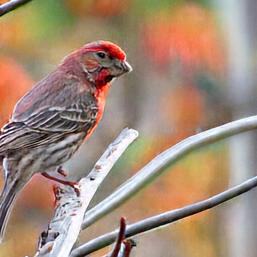
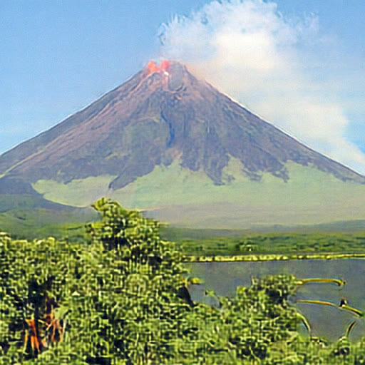
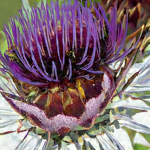
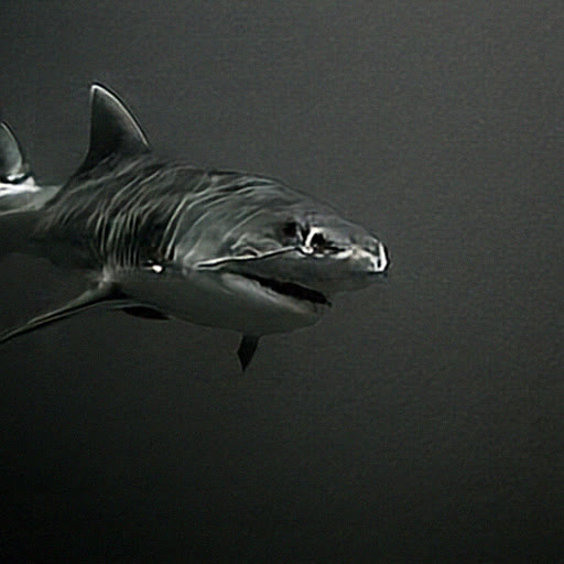
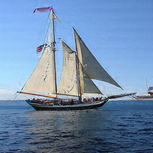
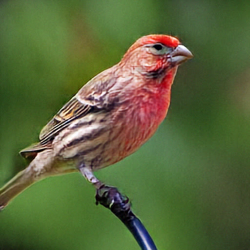
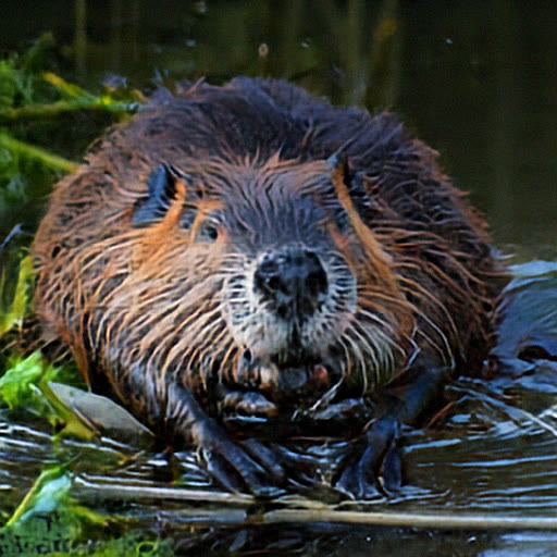
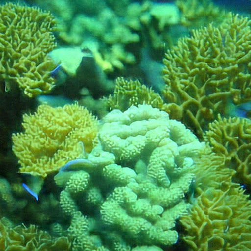
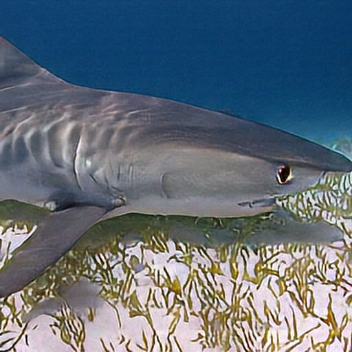
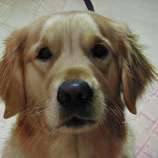
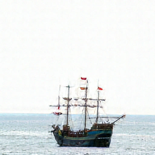
ImageNet 512² samples with the fv-loss
BibTeX
@inproceedings{degeorge2026balancing,
  title     = {Balancing Frequencies and Pixels in Flow Matching},
  author    = {Degeorge, Lucas and Couairon, Paul and Ghosh, Arijit and
               Efros, Alexei A. and Picard, David and Kalogeiton, Vicky},
  booktitle = {Advances in Neural Information Processing Systems (NeurIPS)},
  year      = {2026}
}